
Linear Regression
Linear Functions
Linear are equations with x and y values raised to the power of 1 (usually).
They can be written in Standard Form:
Ax + By = C
Or Slope-Intercept Form:
y = mx + b
Non-Linear Function
Non-Linear Equations have x and y values raised to the power of 2 or more. The functions form wavy lines of some kind but still pass the vertical line test.
Our goal is, given a training set, to learn a function h : X → Y so that h(x) is a “good” predictor for the corresponding value of y. For historical reasons, this function h is called a hypothesis.
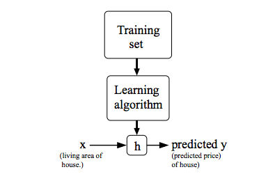 Figure 1 : Model Representation
Linear regression with
onevariable -Univariatelinear regression.
Cost Function
We can measure the accuracy of our hypothesis function by using a cost function. This takes an average difference (actually a fancier version of an average) of all the results of the hypothesis with inputs from X's and the actual output y's.
To break it apart, it is $\frac{1}{2}$ $\bar{x}$ where $\bar{x}$ is the mean of the squares of $h_\theta\left(x_i\right)-y_i$ , or the difference between the predicted value and the actual value.
This function is otherwise called the “Squared error function”, or “Mean squared error”. The mean is halved $\frac{1}{2}$ as a convenience for the computation of the gradient descent, as the derivative term of the square function will cancel out the $\frac{1}{2}$ term. The following image summarizes what the cost function does:
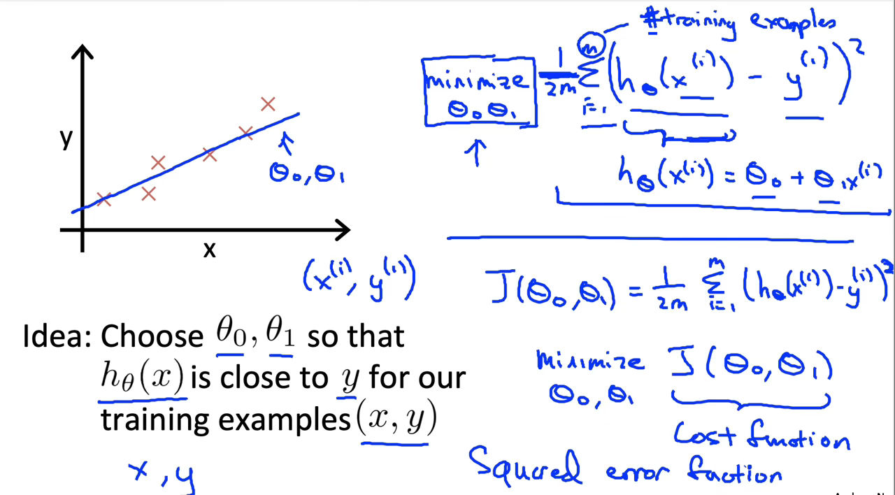 Figure 2 : Cost Function Representation
Cost Function - Intuition I
If we try to think of it in visual terms, our training data set is scattered on the x-y plane. We are trying to make a straight line (defined by $h_\theta\left(x\right)$ which passes through these scattered data points.
Our objective is to get the best possible line. The best possible line will be such so that the average squared vertical distances of the scattered points from the line will be the least. Ideally, the line should pass through all the points of our training data set. In such a case, the value of $J\left(\theta_0, \theta_1\right)$ will be 0. The following example shows the ideal situation where we have a cost function of 0.
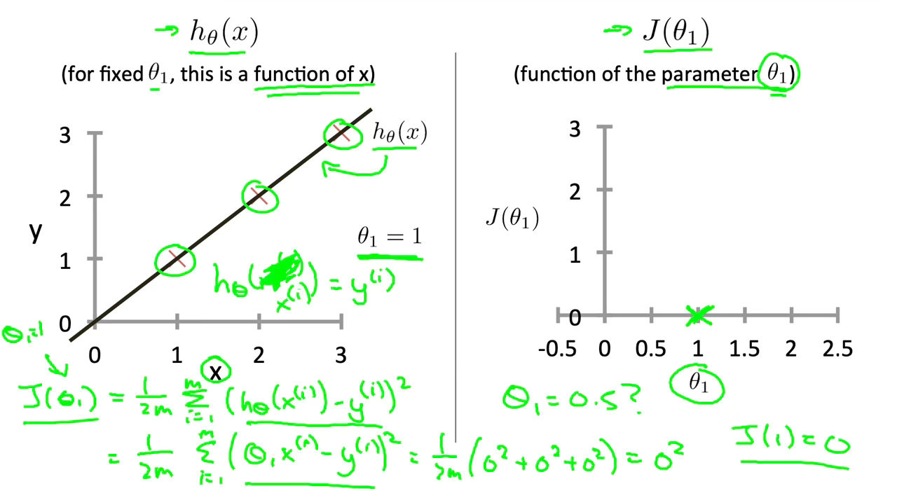 Figure 3 : Cost Function Intuition I
When $\theta_1=1$, we get a slope of 1 which goes through every single data point in our model. Conversely, when $\theta_1$=0.5, we see the vertical distance from our fit to the data points increase.
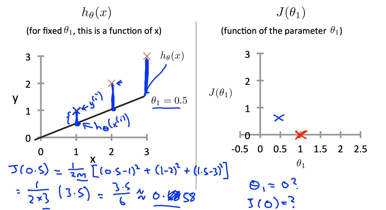 Figure 4 : Cost Function Intuition I
This increases our cost function to 0.58. Plotting several other points yields to the following graph:
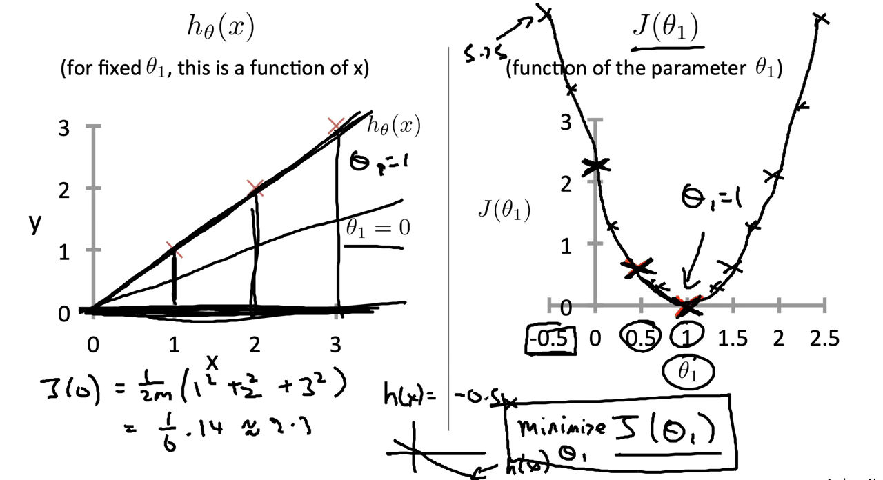 Figure 5 : Cost Function Intuition I
Cost Function - Intuition II
A contour plot is a graph that contains many contour lines. A contour line of a two variable function has a constant value at all points of the same line.
An example of such a graph is the one to the right below.
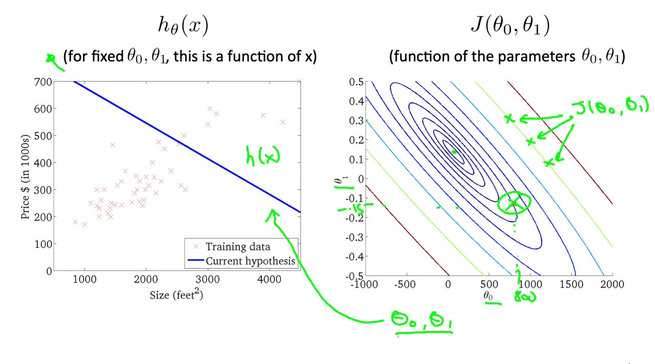 Figure 6 : Cost Function Intuition II
Taking any color and going along the ‘circle’, one would expect to get the same value of the cost function. For example, the three green points found on the green line above have the same value for $J\left(\theta_0, \theta_1\right)$ and as a result, they are found along the same line. The circled x displays the value of the cost function for the graph on the left when $\theta_0$ = 800 and $\theta_1$ = -0.15. Taking another h(x) and plotting its contour plot, one gets the following graphs:
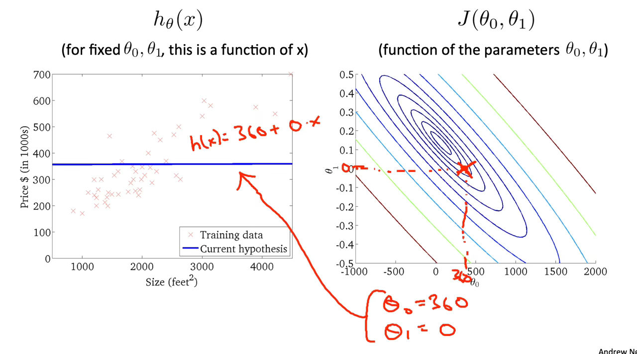 Figure 7 : Cost Function Intuition II
When $\theta_0$ = 360 and $\theta_1$ = 0, the value of $J\left(\theta_0, \theta_1\right)$ in the contour plot gets closer to the center thus reducing the cost function error. Now giving our hypothesis function a slightly positive slope results in a better fit of the data.
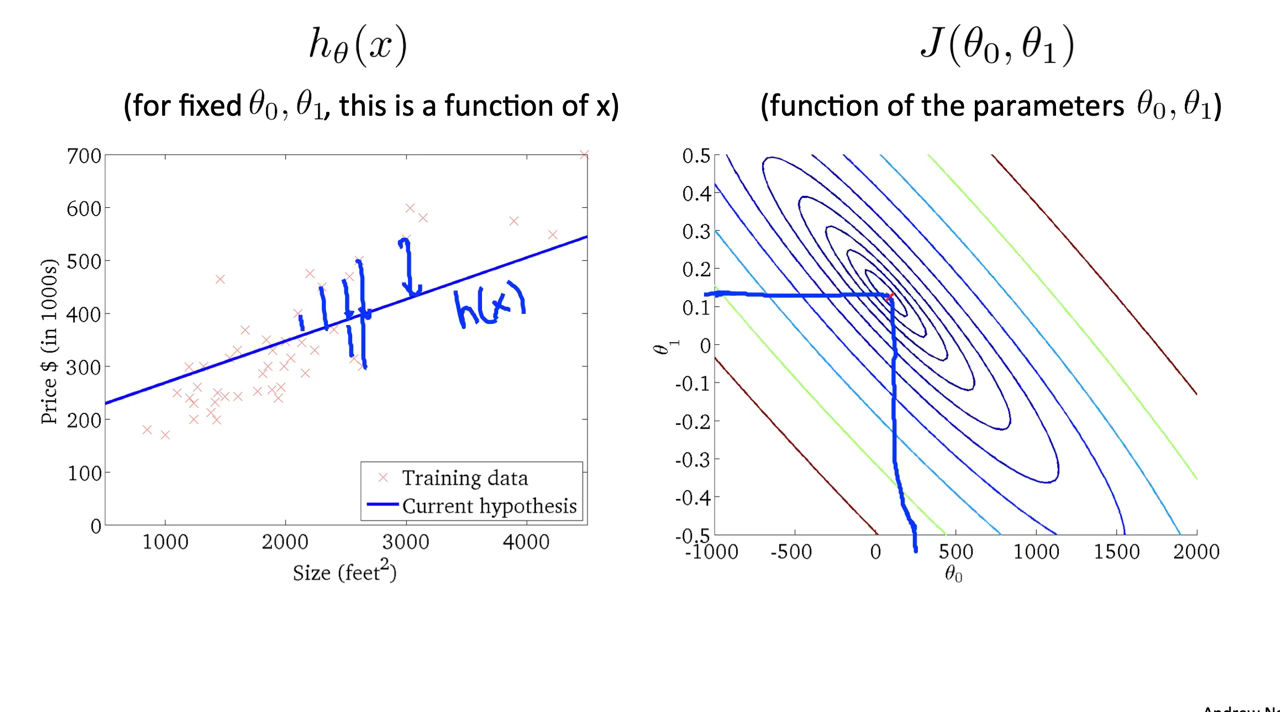 Figure 8 : Cost Function Intuition II
The graph above minimizes the cost function as much as possible and consequently, the result of $\theta_1$ and $\theta_0$ tend to be around 0.12 and 250 respectively. Plotting those values on our graph to the right seems to put our point in the center of the inner most ‘circle’.
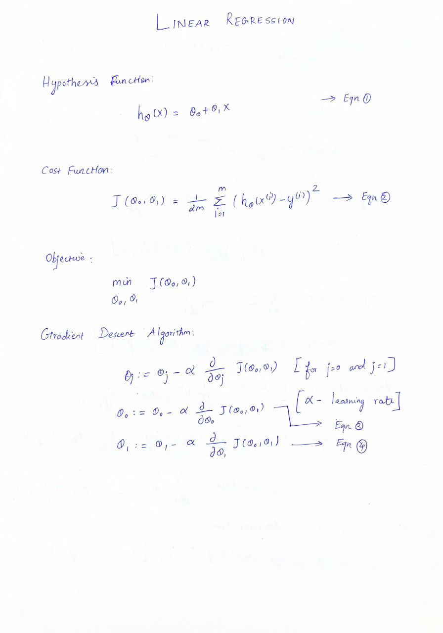
Gradient Descent
\[h_{\theta }(X) = \theta_0 + \theta_1X\]We have our hypothesis function and we have a way of measuring how well it fits into the data. Now we need to estimate the parameters in the hypothesis function. That’s where gradient descent comes in.
Imagine that we graph our hypothesis function based on its fields $\theta_0$ and $\theta_1$ (actually we are graphing the cost function as a function of the parameter estimates). We are not graphing x and y itself, but the parameter range of our hypothesis function and the cost resulting from selecting a particular set of parameters.
We put $\theta_0$ on the x axis and $\theta_1$ on the y axis, with the cost function on the vertical z axis. The points on our graph will be the result of the cost function using our hypothesis with those specific theta parameters. The graph below depicts such a setup.
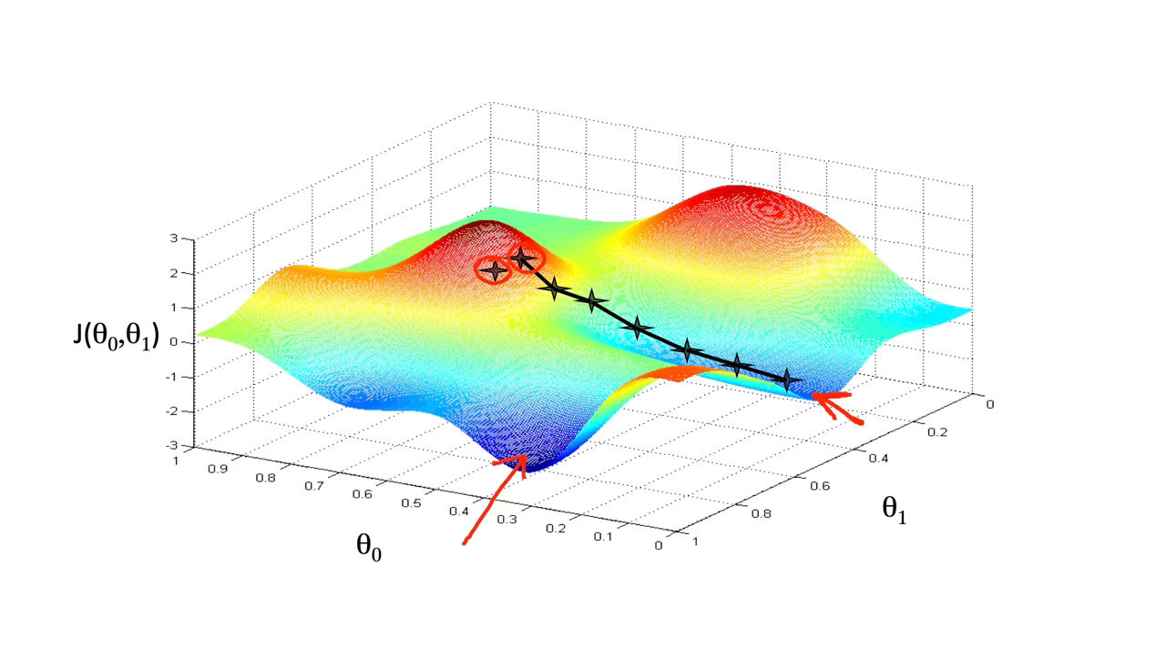 Figure 9 : Gradient Descent
We will know that we have succeeded when our cost function is at the very bottom of the pits in our graph, i.e. when its value is the minimum. The red arrows show the minimum points in the graph.
The way we do this is by taking the derivative (the tangential line to a function) of our cost function. The slope of the tangent is the derivative at that point and it will give us a direction to move towards. We make steps down the cost function in the direction with the steepest descent. The size of each step is determined by the parameter α, which is called the learning rate.
For example, the distance between each ‘star’ in the graph above represents a step determined by our parameter α. A smaller α would result in a smaller step and a larger α results in a larger step. The direction in which the step is taken is determined by the partial derivative of $J\left(\theta_0, \theta_1\right)$. Depending on where one starts on the graph, one could end up at different points. The image above shows us two different starting points that end up in two different places.
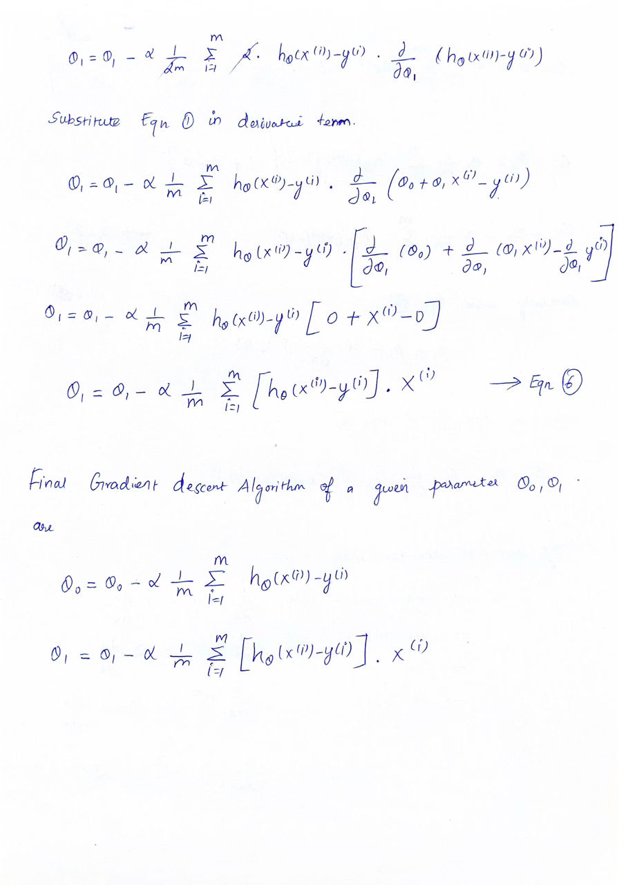
The gradient descent algorithm is:
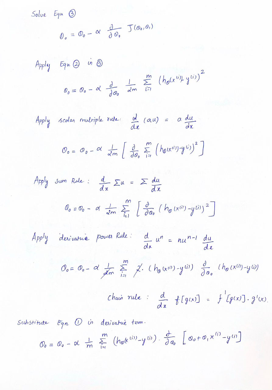
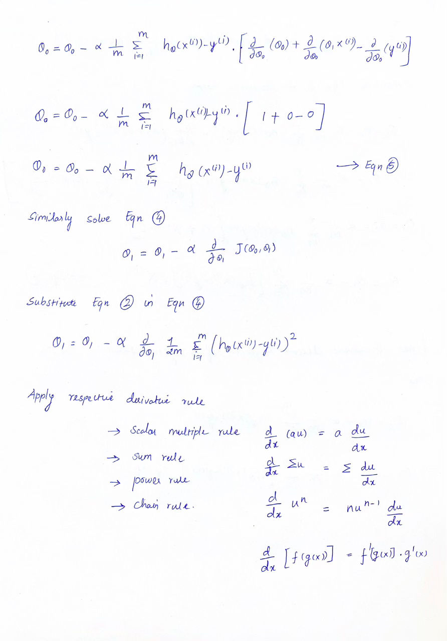
\[\theta_j := \theta_j - \alpha \frac{\partial}{\partial \theta_j} J(\theta_0, \theta_1)\]The derivatives of Gradient Descent Algorithm
References: